Time Series Forecasting Overview¶

Chronos provides both deep learning/machine learning models and traditional statistical models for forecasting.

There’re three ways to do forecasting:

Use highly integrated AutoTS pipeline with auto feature generation, data pre/post-processing, hyperparameter optimization.
Use auto forecasting models with auto hyperparameter optimization.
Use standalone forecasters.

0. Supported Time Series Forecasting Model¶

Model: Model name.
Style: Forecasting model style. Detailed information will be stated in this section.
Multi-Variate: Predict more than one variable at the same time?
Multi-Step: Predict more than one data point in the future?
Exogenous Variables: Take other variables(you don’t need to predict) into consideration?
Distributed: Scale the model to a cluster and take data from distributed file system?
ONNX: Export and use OnnxRuntime to do the inference.
Quantization: Export and use quantized int8 model to do the inference.
Auto Models: AutoModel API support.
AutoTS: AutoTS API support.
Backend: The DL framework we use to implement this model.

Model	Style	Multi-Variate	Multi-Step	Exogenous Variables	Distributed	ONNX	Quantization	Auto Models	AutoTS	Backend
LSTM	RR	✅	❌	✅	✅	✅	✅	✅	✅	pytorch/tf2
Seq2Seq	RR	✅	✅	✅	✅	✅	❌	✅	✅	pytorch/tf2
TCN	RR	✅	✅	✅	✅	✅	✅	✅	✅	pytorch
NBeats	RR	❌	✅	❌	✅	✅	✅	❌	❌	pytorch
MTNet	RR	✅	❌	✅	❌	❌	❌	❌	✳️**	tf2
TCMF	TS	✅	✅	✅	✳️*	❌	❌	❌	❌	pytorch
Prophet	TS	❌	✅	❌	❌	❌	❌	✅	❌	prophet
ARIMA	TS	❌	✅	❌	❌	❌	❌	✅	❌	pmdarima
Customized***	RR	Customized	Customized	Customized	❌	✅	❌	❌	✅	pytorch

* TCMF only partially supports distributed training.
** Auto tuning of MTNet is only supported in our deprecated AutoTS API.
*** Customized model is only supported in AutoTSEstimator with pytorch as backend.

1. Time Series Forecasting Concepts¶

Time series forecasting is one of the most popular tasks on time series data. In short, forecasing aims at predicting the future by using the knowledge you can learn from the history.

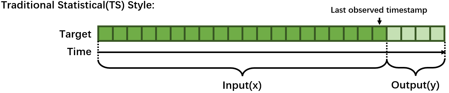
1.1 Traditional Statistical(TS) Style¶

Traditionally, Time series forecasting problem was formulated with rich mathematical fundamentals and statistical models. Typically, one model can only handle one time series and fit on the whole time series before the last observed timestamp and predict the next few steps. Training(fit) is needed every time you change the last observed timestamp.

../../../_images/forecast-TS.png

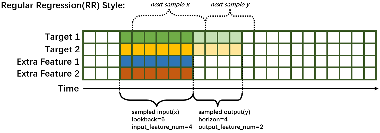
1.2 Regular Regression(RR) Style¶

Recent years, common deep learning architectures (e.g. RNN, CNN, Transformer, etc.) are being successfully applied to forecasting problem. Forecasting is transformed to a supervised learning regression problem in this style. A model can predict several time series. Typically, a sampling process based on sliding-window is needed, some terminology is explained as following:

lookback / past_seq_len: the length of historical data along time. This number is tunable.
horizon / future_seq_len: the length of predicted data along time. This number is depended on the task definition. If this value larger than 1, then the forecasting task is Multi-Step.
input_feature_num: The number of variables the model can observe. This number is tunable since we can select a subset of extra feature to use.
output_feature_num: The number of variables the model to predict. This number is depended on the task definition. If this value larger than 1, then the forecasting task is Multi-Variate.

../../../_images/forecast-RR.png

2. Use AutoTS Pipeline¶

For AutoTS Pipeline, we will leverage AutoTSEstimator, TSPipeline and preferably TSDataset. A typical usage of AutoTS pipeline basically contains 3 steps.

Prepare a TSDataset or customized data creator.
Init a AutoTSEstimator and call .fit() on the data.
Use the returned TSPipeline for further development.

Warning

AutoTSTrainer workflow has been deprecated, no feature updates or performance improvement will be carried out. Users of AutoTSTrainer may refer to Chronos API doc.

Note

AutoTSEstimator currently only support pytorch backend.

View Quick Start for a more detailed example.

2.1 Prepare dataset¶

AutoTSEstimator support 2 types of data input.

You can easily prepare your data in TSDataset (recommended). You may refer to here for the detailed information to prepare your TSDataset with proper data processing and feature generation. Here is a typical TSDataset preparation.

from bigdl.chronos.data import TSDataset
from sklearn.preprocessing import StandardScaler

tsdata_train, tsdata_val, tsdata_test\
    = TSDataset.from_pandas(df, dt_col="timestamp", target_col="value", with_split=True, val_ratio=0.1, test_ratio=0.1)

standard_scaler = StandardScaler()
for tsdata in [tsdata_train, tsdata_val, tsdata_test]:
    tsdata.gen_dt_feature()\
          .impute(mode="last")\
          .scale(standard_scaler, fit=(tsdata is tsdata_train))

You can also create your own data creator. The data creator takes a dictionary config and returns a pytorch dataloader. Users may define their own customized key and add them to the search space. “batch_size” is the only fixed key.

from torch.utils.data import DataLoader
def training_data_creator(config):
    return Dataloader(..., batch_size=config['batch_size'])

2.2 Create an AutoTSEstimator¶

AutoTSEstimator depends on the Distributed Hyper-parameter Tuning supported by Project Orca. It also provides time series only functionalities and optimization. Here is a typical initialization process.

import bigdl.orca.automl.hp as hp
from bigdl.chronos.autots import AutoTSEstimator
auto_estimator = AutoTSEstimator(model='lstm',
                                 search_space='normal',
                                 past_seq_len=hp.randint(1, 10),
                                 future_seq_len=1,
                                 selected_features="auto") 

We prebuild three defualt search space for each build-in model, which you can use the by setting search_space to “minimal”，”normal”, or “large” or define your own search space in a dictionary. The larger the search space, the better accuracy you will get and the more time will be cost.

past_seq_len can be set as a hp sample function, the proper range is highly related to your data. A range between 0.5 cycle and 2 cycle is reasonable. You may set it to "auto", then a cycle length will be detected automatically and this parameter will be set to a random search between 0.5 cycle and 2 cycle length.

selected_features is set to "auto" by default, where the AutoTSEstimator will find the best subset of extra features to help the forecasting task.

2.3 Fit on AutoTSEstimator¶

Fitting on AutoTSEstimator is fairly easy. A TSPipeline will be returned once fitting is completed.

ts_pipeline = auto_estimator.fit(data=tsdata_train,
                                 validation_data=tsdata_val,
                                 batch_size=hp.randint(32, 64),
                                 epochs=5)

Detailed information and settings please refer to AutoTSEstimator API doc.

2.4 Development on TSPipeline¶

You may carry out predict, evaluate, incremental training or save/load for further development.

# predict with the best trial
y_pred = ts_pipeline.predict(tsdata_test)

# evaluate the result pipeline
mse, smape = ts_pipeline.evaluate(tsdata_test, metrics=["mse", "smape"])
print("Evaluate: the mean square error is", mse)
print("Evaluate: the smape value is", smape)

# save the pipeline
my_ppl_file_path = "/tmp/saved_pipeline"
ts_pipeline.save(my_ppl_file_path)

# restore the pipeline for further deployment
from bigdl.chronos.autots import TSPipeline
loaded_ppl = TSPipeline.load(my_ppl_file_path)

Detailed information please refer to TSPipeline API doc.

Note

init_orca_context is not needed if you just use the trained TSPipeline for inference, evaluation or incremental fitting.

Note

Incremental fitting on TSPipeline just update the model weights the standard way, which does not involve AutoML.

3. Use Standalone Forecaster Pipeline¶

Chronos provides a set of standalone time series forecasters without AutoML support, including deep learning models as well as traditional statistical models.

View some examples notebooks for Network Traffic Prediction

The common process of using a Forecaster looks like below.

# set fixed hyperparameters, loss, metric...
f = Forecaster(...)
# input data, batch size, epoch...
f.fit(...)
# input test data x, batch size...
f.predict(...)

The input data can be easily get from TSDataset. View Quick Start for a more detailed example. Refer to API docs of each Forecaster for detailed usage instructions and examples.

3.1 LSTMForecaster¶

LSTMForecaster wraps a vanilla LSTM model, and is suitable for univariate time series forecasting.

View Network Traffic Prediction notebook and LSTMForecaster API Doc for more details.

3.2 Seq2SeqForecaster¶

Seq2SeqForecaster wraps a sequence to sequence model based on LSTM, and is suitable for multivariant & multistep time series forecasting.

View Seq2SeqForecaster API Doc for more details.

3.3 TCNForecaster¶

Temporal Convolutional Networks (TCN) is a neural network that use convolutional architecture rather than recurrent networks. It supports multi-step and multi-variant cases. Causal Convolutions enables large scale parallel computing which makes TCN has less inference time than RNN based model such as LSTM.

View Network Traffic multivariate multistep Prediction notebook and TCNForecaster API Doc for more details.

3.4 MTNetForecaster¶

Note

Additional Dependencies: You need to install bigdl-nano[tensorflow] to enable this built-in model.

pip install bigdl-nano[tensorflow]

MTNetForecaster wraps a MTNet model. The model architecture mostly follows the MTNet paper with slight modifications, and is suitable for multivariate time series forecasting.

View Network Traffic Prediction notebook and MTNetForecaster API Doc for more details.

3.5 TCMFForecaster¶

TCMFForecaster wraps a model architecture that follows implementation of the paper DeepGLO paper with slight modifications. It is especially suitable for extremely high dimensional (up-to millions) multivariate time series forecasting.

View High-dimensional Electricity Data Forecasting example and TCMFForecaster API Doc for more details.

3.6 ARIMAForecaster¶

Note

Additional Dependencies: You need to install pmdarima to enable this built-in model.

pip install pmdarima==1.8.5

ARIMAForecaster wraps a ARIMA model and is suitable for univariate time series forecasting. It works best with data that show evidence of non-stationarity in the sense of mean (and an initial differencing step (corresponding to the “I, integrated” part of the model) can be applied one or more times to eliminate the non-stationarity of the mean function.

View ARIMAForecaster API Doc for more details.

3.7 ProphetForecaster¶

Note

Additional Dependencies: You need to install prophet to enable this built-in model.

pip install prophet==1.1.0

Note

Acceleration Note: Intel® Distribution for Python may improve the speed of prophet’s training and inferencing. You may install it by refering to https://www.intel.com/content/www/us/en/developer/tools/oneapi/distribution-for-python.html.

ProphetForecaster wraps the Prophet model (site) which is an additive model where non-linear trends are fit with yearly, weekly, and daily seasonality, plus holiday effects and is suitable for univariate time series forecasting. It works best with time series that have strong seasonal effects and several seasons of historical data and is robust to missing data and shifts in the trend, and typically handles outliers well.

View Stock Prediction notebook and ProphetForecaster API Doc for more details.

3.8 NBeatsForecaster¶

Neural basis expansion analysis for interpretable time series forecasting (N-BEATS) is a deep neural architecture based on backward and forward residual links and a very deep stack of fully-connected layers. Nbeats can solve univariate time series point forecasting problems, being interpretable, and fast to train.

4. Use Auto forecasting model¶

Auto forecasting models are designed to be used exactly the same as Forecasters. The only difference is that you can set hp search function to the hyperparameters and the .fit() method will search the best hyperparameter setting.

# set hyperparameters in hp search function, loss, metric...
auto_model = AutoModel(...)
# input data, batch size, epoch...
auto_model.fit(...)
# input test data x, batch size...
auto_model.predict(...)

The input data can be easily get from TSDataset. Users can refer to detailed API doc.